#Python Pandas – Find difference between two data frames | Explore Tumblr posts and blogs

dpikablog · 6 years ago

Text

Week 1 Assignment – Running an Analysis of variance (ANOVA)

Objective:

The assignment of the week deals with Analysis of variance. Given a dataset some form of Statistical Analysis test to be performed to check and evaluate its Statistical significance.

Before getting into the crux of the problem let us understand some of the important concepts

Hypothesis testing - It is one of the most important Inferential Statistics where the hypothesis is performed on the sample data from a larger population. Hypothesis testing is a statistical assumption taken by an analyst on the nature of the data and its reason for analysis. In other words, Statistical Hypothesis testing assesses evidence provided by data in favour of or against each hypothesis about the problem.

There are two types of Hypothesis

Null Hypothesis – The null hypothesis is assumed to be true until evidence indicate otherwise. The general assumptions made on the data (people with depression are more likely to smoke)

Alternate Hypothesis – Once stronger evidences are made, one can reject Null hypothesis and accept Alternate hypothesis (One needs to come with strong evidence to challenge the null hypothesis and draw proper conclusions).In this case one needs to show evidences such that there is no relation between people smoking and their depression levels

Example:

The Null hypothesis is that the number of cigarettes smoked by the person is dependent on the person’s depression level. Based on the p-value we make conclusions either to accept the null hypothesis or fail to accept the null hypothesis(accept alternative hypothesis)

Steps involved in Hypothesis testing:

1. Choose the Null hypothesis (H0 ) and alternate hypothesis (Ha)

2. Choose the sample

3. Assess the evidence

4. Draw the conclusions

The Null hypothesis is accepted/rejected based on the p-value significance level of test

If p<= 0.05, then reject the null hypothesis (accept the alternate hypothesis)

If p > 0.05 null hypothesis is accepted

Wrongly rejecting the null hypothesis leads to type one error

Sampling variability:

The measures of the sample (subset of population) varying from the measures of the population is called Sampling variability. In other words sample results changing from sample to sample.

Central Limit theorem:

As long as adequately large samples and an adequately large number of samples are used from a population,the distribution of the statistics of the sample will be normally distributed. In other words, the more the sample the accurate it is to the population parameters.

Choosing Statistical test:

Please find the below tabulation to identify what test can be done at a given condition. Some of the statistical tools used for this are

Chi-square test of independence, ANOVA- Analysis of variance, correlation coefficient.

Explanatory variables are input or independent variable And response variable is the output variable or dependent variable.

Explanatory Response Type of test

Categorical Categorical Chi-square test

Quantitative Quantitative Pearson correlation

Categorical Quantitative ANOVA

Quantitative Categorical Chi-square test

ANOVA:

Anova F test, helps to identify, Are the difference among the sample means due to true difference among the population or merely due to sampling variability.

F = variation among sample means / by variations within groups

Let’s implement our learning in python.

The Null hypothesis here is smoking and depression levels are unrelated

The Alternate hypothesis is smoking and depression levels are related.

# importing required libraries

import numpy as np

import pandas as pd

import statsmodels.formula.api as smf

data = pd.read_csv("my_data...nesarc.csv",low_memory=False)

#setting variables you will be working with to numeric

data['S3AQ3B1'] = data['S3AQ3B1'].convert_objects(convert_numeric=True)

#data['S3AQ3B1'] = pd.to_numeric(data.S3AQ3B1)

data['S3AQ3C1'] = data['S3AQ3C1'].convert_objects(convert_numeric=True)

#data['S3AQ3C1'] = pd.to_numeric(data.S3AQ3C1)

data['CHECK321'] = data['CHECK321'].convert_objects(convert_numeric=True)

#data['CHECK321'] = pd.to_numeric(data.CHECK321)

#subset data to young adults age 18 to 25 who have smoked in the past 12 months

sub1=data[(data['AGE']>=18) & (data['AGE']<=25) & (data['CHECK321']==1)]

#SETTING MISSING DATA

sub1['S3AQ3B1']=sub1['S3AQ3B1'].replace(9, np.nan)

sub1['S3AQ3C1']=sub1['S3AQ3C1'].replace(99, np.nan)

#recoding number of days smoked in the past month

recode1 = {1: 30, 2: 22, 3: 14, 4: 5, 5: 2.5, 6: 1}

sub1['USFREQMO']= sub1['S3AQ3B1'].map(recode1)

#converting new variable USFREQMMO to numeric

sub1['USFREQMO']= sub1['USFREQMO'].convert_objects(convert_numeric=True)

# Creating a secondary variable multiplying the days smoked/month and the number of cig/per day

sub1['NUMCIGMO_EST']=sub1['USFREQMO'] * sub1['S3AQ3C1']

sub1['NUMCIGMO_EST']= sub1['NUMCIGMO_EST'].convert_objects(convert_numeric=True)

ct1 = sub1.groupby('NUMCIGMO_EST').size()

print (ct1)

print(sub1['MAJORDEPLIFE'])

# using ols function for calculating the F-statistic and associated p value

The ols is the ordinary least square function takes the response variable NUMCIGMO_EST and its explanatory variable MAJORDEPLIFE, C is indicated to specify that it’s a categorical variable.

model1 = smf.ols(formula='NUMCIGMO_EST ~ C(MAJORDEPLIFE)', data=sub1)

results1 = model1.fit()

print (results1.summary())

Inference – Since the p value is greater than 0.05, we accept the null hypothesis that the sample means are statistically equal. And there is no association between depression levels and cigarette smoked.

sub2 = sub1[['NUMCIGMO_EST', 'MAJORDEPLIFE']].dropna()

print ('means for numcigmo_est by major depression status')

m1= sub2.groupby('MAJORDEPLIFE').mean()

print (m1)

print ('standard deviations for numcigmo_est by major depression status')

sd1 = sub2.groupby('MAJORDEPLIFE').std()

print (sd1)

Since the null hypothesis is true we conclude that the sample mean and standard deviation of the two samples are statistically equal. From the sample statistics we infer that the depression levels and smoking are unrelated to each other

Till now, we ran the ANOVA test for two levels of the categorical variable(MAJORDEPLIFE, 0,1) Lets now look at the categorical variable(ETHRACE2A,White, Black, American Indian, Asian native and Latino) having five levels and see how the differences in the mean are captured.

The problem here is, The F-statistic and ‘p’ value does not provide any insight as to why the null hypothesis is rejected when there are multiple levels in categorical Explanatory variable.

The significant ANOVA does not tell which groups are different from the others. To determine this we would need to perform post-hoc test for ANOVA

Why Post-hoc tests for ANOVA?

Post hoc test known as after analysis test, This is performed to prevent excessive Type one error. Not implementing this leads to family wise error rate, given by the formula

FWE = 1 – (1 – αIT)C

Where:

αIT = alpha level for an individual test (e.g. .05),

c = Number of comparisons.

Post-hoc tests are designed to evaluate the difference between the pair of means while protecting against inflation of type one error.

Let’s continue the code to perform post-hoc test.

# Importing the library

Import statsmodels.stats.multicomp as multi

# adding the variable of interest to a separate data frame

sub3 = sub1[['NUMCIGMO_EST', 'ETHRACE2A']].dropna()

# calling the ols function and passing the explanatory categorical and response variable

model2 = smf.ols(formula='NUMCIGMO_EST ~ C(ETHRACE2A)', data=sub3).fit()

print(model2.summary())

print ('means for numcigmo_est by major depression status')

m2= sub3.groupby('ETHRACE2A').mean()

print(m2)

print('standard deviations for numcigmo_est by major depression status')

sd2 = sub3.groupby('ETHRACE2A').std()

print(sd2)

# Include required parameters in the MultiComparison function and then run the post-hoc TukeyHSD test

mc1 = multi.MultiComparison(sub3['NUMCIGMO_EST'], sub3['ETHRACE2A'])

res1 = mc1.tukeyhsd()

print(res1.summary())

#statistics ANOVA DataAnalysis

1 note · View note

360digitmgba · 5 years ago

Text

Python in Shaping the Future of Machine Learning 5

How Amazon Is Dazzling The World With Ai & Ml

You can use either of them, as both give just about the same outcomes specifically in case of CART analytics as shown in below determination. Entropy in simpler terms is the measure of randomness or uncertainty.

In the above example, a choice tree is being used for a classification drawback to resolve whether an individual is fit or unit. The depth of the tree is referred to the length of the tree from root node to leaf. If you could have disposable revenue to spend then I’d highly recommend hiring a mentor who can stroll you through your issues. Income share mentorships make new opportunities accessible to people who can’t afford the professional time or discover professional knowledge scientists to be taught from.

” There are many assets across the net, but I don’t wish to give anyone the mistaken impression that the path to data science is as simple as taking a few MOOCs. Unless you have already got a robust quantitative background, the highway to becoming a knowledge scientist might be challenging but not inconceivable. A knowledge scientist will never thrive if he/she doesn’t understand what to take a look at to run when and the way to interpret their findings.

Stock Market Clustering Project — In this project, you'll use a K-means clustering algorithm to establish related corporations by discovering correlations amongst inventory market actions over a given time span. We have tried to take an extra thrilling approach to Machine Learning, by not working on simply the idea of it, however as a substitute by using the technology to actually build actual-world initiatives that you should use. Furthermore, you will learn how to write the codes after which see them in motion and actually learn to assume like a machine studying skilled. In this weblog, we'll take a look at initiatives divided largely into two totally different levels i.e. First, projects talked about under the beginner heading cover important ideas of a specific technique/algorithm.

But that is the proper guide for superior-intermediate to professional data scientists. If you need to know how to work professionally as a knowledge scientist, this guide is for you. But this is only for intermediate, advanced, and skilled knowledge scientists since you have to know the fundamentals before starting on this guide. P is the likelihood of a knowledge level belonging to class 1 as predicted by the model.

And check out the top 5 rows utilizing the head() Pandas DataFrame perform. This is how the K Nearest Neighbours algorithm works in principle. As you possibly can see, visualizing the data is a big assist to get an intuitive picture of what the k values must be. Finally, we return a category as output which is closest to the new knowledge level, in accordance with various measures. The measures used include Euclidean distance amongst others.

Now that we now have defined our phrases, let’s move to the lessons of Machine Learning or ML algorithms. The why must be predicted using the ML mannequin trained on the seen knowledge. The predicted variable is often known as the dependent variable. For example, information of a thousand customers with their age, gender, time of entry and exit and their purchases. The subsequent question I all the time get is, “What can I do to develop these abilities?

youtube

Experienced working with skilled builders could make or break your capability to land a knowledge science position. Learning knowledge science will never be straightforward without any assistance from the community or from somebody who's prepared to help novices. These someones are the ones which might be making up our wonderful LinkedIn Data Science Community.

Similarly, tasks beneath superior class contain the application of multiple algorithms along with key ideas to achieve the answer of the problem at hand. Thus, we have designed a comprehensive listing of projects in the Machine Learning course that offers a palms-on experience with ML and how to construct precise initiatives using the Machine Learning algorithms. Furthermore, this course is an observation up to our Introduction to Machine Learning course and delves further deeper into the sensible applications of Machine Learning. Changes aren't just challenges, they are additionally alternatives for much higher-paying and much much less laborious jobs than the roles you hold at present. And, if by probability, you happen to be a scholar studying this article, you now know which business you should concentrate on – fully. All the best, and bear in mind to benefit from the process of studying.

Regardless of your age, that is the best time to be alive – ever. Because area knowledge is out there extra widely today than at any time up to now. And make the right selections at the right instances – and no, it's never too late when you're high quality trainers able to mentor you. May the fun of studying a completely new idea with really enlightened insight never leave you. Dimensionless.in is an elite information science training firm that imparts trade degree expertise and knowledge to those with an actual thirst to study. Training is given from the fundamentals, resulting in a strong basis.

If you need to be an information scientist, not having a decent Kaggle profile is inexcusable. Kaggle will be like a showcase of your information science expertise to the whole world. Even when you don’t rank very excessive, consistency and practice can get you there most of the time. This single book incorporates a number of the latest and the most effective methods to attain what you should be a professional information scientist. Every chapter has multiple case research taken from the experiences within the industry.Vincent Granville is recognized worldwide as probably the greatest-recognized useful resource in information science. The level is slightly advanced, and it is not beneficial for novices.

The greatest potential break up will be the one with the lowest general entropy. This is because of decreased entropy, lower uncertainty and hence more probability. Dropping the variables that are of least importance in deciding. In Titanic dataset columns such as name, cabin no. ticket no. is of least importance. Decision Trees can be utilized for classification as well as regression problems. That’s why they are called Classification or Regression Trees.

Therefore, our prediction could be that the unseen flower is a Rose. Notice that our prior probabilities of both the lessons favoured Sunflower. But as soon as we factored the data about thorns, our decision changed. For all N factors, we sum the squares of the distinction of the predicted value of Y by the model, i.e. Y’ and the precise worth of the anticipated variable for that point, i.e.

They want a stable understanding of algebra and calculus. In good old days, Math was a subject based mostly on common sense and the necessity to resolve primary issues based on logic. This hasn’t modified a lot, though the size has blown up exponentially. A statistical sensibility provides a stable foundation for several evaluation tools and methods, that are utilized by a knowledge scientist to build their fashions and analytic routines. An information scientist is not going to conclude, decide, or resolve without enough data.

This is the essence of the ML algorithm that platforms such as Amazon and Flipkart use for each customer. Their algorithms are much more complex, but that is their essence. Determine sort of characteristic capabilities decide whether a kind of feature is categorical or continuous. There are 2 criterias for the function to be known as categorical, first if the feature is of knowledge sort string and second, the no. of categories for the function is less than 10. I actually have used Information Gain Entropy as a measure of impurity.

With the right strategy and by trying at the right corners, you'll find information scientist mentors who might help you bridge the hole between theoretical and sensible functions of data science. Development of algorithms for Computer Aided Detection of early-stage breast most cancers among others. KKD cup is a well-liked knowledge mining and knowledge discovery competition held annually. It is likely one of the first-ever data science competitors which dates again to 1997. With the growing demand to research giant amounts of data inside small time frames, organizations choose working with the data immediately over samples. Consequently, this presents a herculean task for an information scientist with a limitation of time. Sports Betting… Predict field scores given the info available at the time proper before each new recreation.

Regression analysis is a type of predictive modeling method which investigates the relationship between dependent and independent variables. Regression goals at finding a straight line which may accurately depict the precise relationship between the 2 variables. Data is rising day by day, and it is unimaginable to understand all of the knowledge with higher velocity and higher accuracy. More than 80% of the information is unstructured that's audios, movies, photographs, paperwork, graphs, and so on. Finding patterns in knowledge on planet earth is impossible for human brains. The knowledge has been very large and the time taken to compute would improve solely. This is the place Machine Learning comes into motion, to help people with significant information in minimum time.

It may be proven that there isn't an absolute “best” criterion which would be independent of the final goal of the clustering. Consequently, it is the consumer which should supply this criterion, in such a means that the results of the clustering will go well with their needs. Clustering is likely one of the most important unsupervised learning problems; so, like each other's downside of this kind, it deals with finding a structure in a collection of unlabeled information.

In this article, we shall be looking at why there's even a necessity for people to have mentors in knowledge science and the way we can discover them. Although Data Science has been around us ever since the 1960s, it has only gained traction in the previous couple of a long time. This is one of the major reasons why budding knowledge scientists find it quite challenging to find the best mentors.

Now, anybody with discipline and persistence can study information science and turn out to be a data scientist. The coaching obtained is customized to cater to the needs of each pupil. These days, just having an impressive profile on Kaggle might be enough to land you a job interview at the very least. Kaggle is a site that has been hosting information science competitions for a few years. The competition is immense and intense, however so are the tutorials and the articles are additionally equally highly effective and instructive.

Explore more on Data Science Course In Hyderabad

360DigiTMG - Data Analytics, Data Science Course Training Hyderabad

Address:-2-56/2/19, 3rd floor,, Vijaya towers, near Meridian school,, Ayyappa Society Rd, Madhapur,, Hyderabad, Telangana 500081

#Python in Shaping the Future of Machine Learning 5

0 notes

itsrahulpradeepposts · 5 years ago

Text

Why Python is used in data science? How data science courses help in a successful career post COVID pandemic?

Data science has tremendous growth opportunities and is one of the hot careers in the current world. Many businesses are thriving for skilled data scientists. Data science requires many skills to become an expert – One of the important skills is Python programming. Python is a programming language widely used in many fields. It is considered as the king of the coding world. Data scientists extensively use this language and even beginners find it easy to learn the Python language. To learn this language, there are many Python data science courses that guide and train you in an effective way.

What is Python?

Python is an interpreted and object-oriented programming language. It is an easily understandable language whose syntaxes can be grasped by a beginner quickly. It was found by Guido in 1991. It is supported in operating systems like Linux, Windows, macOS, and a lot more. The Python is developed and managed by the Python software foundation.

The second version of Python was released in 2000. It features list comprehension and reference counting. This version was officially stopped functioning in 2020. Currently, only the Python version 3.5x and later versions are supported.

Why Python is used in data science?

Python is the most preferred programming language by the data scientists as it effectively resolves tasks. It is one of the top data science tools used in various industries. It is an ideal language to implement algorithms. Python’s scikit-learn is a vital tool that the data scientist find it useful while solving many machine learning tasks. Data science uses Python libraries to solve a task.

Python is very good when it comes to scalability. It gives you flexibility and multiple solutions for different problems. It is faster than Matlab. The main reason why YouTube started working in Python is because of its exceptional scalability.

Features of Python language

Python has a syntax that can be understood easily.

It has a vast library and community support.

We can easily test codes as it has interactive modes.

The errors that arise can be easily understood and cleared quickly.

It is free software, and it can be downloaded online. Even there are free online Python compilers available.

The code can be extended by adding modules. These modules can also be implemented in other languages like C, C++, etc.

It offers a programmable interface as it is expressive in nature.

We can code Python anywhere.

The access to this language is simple. So we can easily make the program working.

The different types of Python libraries used for data science

1.Matplotlib

Matplotlib is used for effective data visualization. It is used to develop line graphs, pie charts, histograms efficiently. It has interactive features like zooming and planning the data in graphics format. The analysis and visualization of data are vital for a company. This library helps to complete the work efficiently.

2.NumPy

NumPy is a library that stands for Numerical Python. As the name suggests, it does statistical and mathematical functions that effectively handles a large n-array. This helps in improving the data and execution rate.

3.Scikit-learn

Scikit- learn is a data science tool used for machine learning. It provides many algorithms and functions that help the user through a constant interface. Therefore, it offers active data sets and capable of solving real-time problems more efficiently.

4.Pandas

Pandas is a library that is used for data analysis and manipulation. Even though the data to be manipulated is large, it does the manipulation job easily and quickly. It is an absolute best tool for data wrangling. It has two types of data structures .i.e. series, and data frame. Series takes care of one-dimensional data, and the data frame takes care of two-dimensional data.

5.Scipy

Scipy is a popular library majorly used in the data science field. It basically does scientific computation. It contains many sub-modules used primarily in science and engineering fields for FFT, signal, image processing, optimization, integration, interpolation, linear algebra, ODE solvers, etc.

Importance of data science

Data scientists are becoming more important for a company in the 21st century. They are becoming a significant factor in public agencies, private companies, trades, products and non-profit organizations. A data scientist plays as a curator, software programmer, computer scientist, etc. They are the central part of managing the collection of digital data. According to our analysis, we have listed below the major reasons why data science is important in developing the world’s economy.

Data science helps to create a relationship between the company and the client. This connection helps to know the customer’s requirements and work accordingly.

Data scientists are the base for the functioning and the growth of any product. Thus they become an important part as they are involved in doing significant tasks .i.e. data analysis and problem-solving.

There is a vast amount of data travelling around the world and if it is used efficiently, it results in the successful growth of the product.

The resulting products have a storytelling capability that creates a reliable connection among the customers. This is one of the reasons why data science is popular.

It can be applied to various industries like health-care, travel, software companies, etc.

Big data analytics is majorly used to solve the complexities and find a solution for the problems in IT companies, resource management, and human resource.

It greatly influences the retail or local sellers. Currently, due to the emergence of many supermarkets and shops, the customers approaching the retail sellers are drastically decreased. Thus data analytics helps to build a connection between the customers and local sellers.

Are you finding it difficult to answer the questions in an interview? Here are some frequently asked data science interview questions on basic concepts

Q. How to maintain a deployed model?

To maintain a deployed model, we have to

Monitor

Evaluate

Compare

Rebuild

Q. What is random forest model?

Random forest model consists of several decision trees. If you split the data into different sections and assign each group of data a decision tree, the random forest models combine all the trees.

Q. What are recommendation systems?

A recommendation system recommends the products to the users based on their previous purchases or preferences. There are mainly two areas .i.e. collaborative filtering and content-based filtering.

Q. Explain the significance of p-value?

P-value <= 0.5 : rejects the null-hypothesis

P-value > 0.5 : accepts null-hypothesis

P-value = 0.5 : it will either except or deny the null-hypothesis

Q. What is logistic regression?

Logistic regression is a method to obtain a binary result from a linear combination of predictor variables.

Q. What are the steps in building a decision tree?

Take the full data as the input.

Split the dataset in such a way that the separation of the class is maximum.

Split the input.

Follow steps 1 and 2 to the separated data again.

Stop this process after the complete data is separated.

Best Python data science courses

Many websites provide Data Science online courses. Here are the best sites that offer data science training based on Python.

GreatLearning

Coursera

EdX

Alison

Udacity

Skillathon

Konvinity

Simplilearn

How data science courses help in a successful career post-COVID-19 pandemic?

The economic downfall due to COVID-19 impacts has lead to upskill oneself as the world scenarios are changing drastically. Adding skills to your resume gives an added advantage of getting a job easily. The businesses are going to invest mainly in two domains .i.e. data analysis of customer’s demand and understanding the business numbers. It is nearly impossible to master in data science, but this lockdown may help you become a professional by indulging in data science programs.

Firstly, start searching for the best data science course on the internet. Secondly, make a master plan in such a way that you complete all the courses successfully. Many short-term courses are there online that are similar to the regular courses, but you can complete it within a few days. For example, Analytix Labs are providing these kinds of courses to upskill yourself. So this is the right time where you are free without any work and passing time. You can use this time efficiently by enrolling in these courses and become more skilled in data science than before. These course providers also give a data science certification for the course you did; this will help to build your resume.

Data science is a versatile field that has a broad scope in the current world. These data scientists are the ones who are the pillars of businesses. They use various factors like programming languages, machine learning, and statistics in solving a real-world problem. When it comes to programming languages, it is best to learn Python as it is easy to understand and has an interactive interface. Make efficient use of time in COVID-19 lockdown to upskill and build yourself.

#data science #greatlearning #python #online course #career

0 notes

t-baba · 8 years ago

Photo

Pandas: The Swiss Army Knife for Your Data, Part 2

This is part two of a two-part tutorial about Pandas, the amazing Python data analytics toolkit.

In part one, we covered the basic data types of Pandas: the series and the data frame. We imported and exported data, selected subsets of data, worked with metadata, and sorted the data.

In this part, we'll continue our journey and deal with missing data, data manipulation, data merging, data grouping, time series, and plotting.

Dealing With Missing Values

One of the strongest points of pandas is its handling of missing values. It will not just crash and burn in the presence of missing data. When data is missing, pandas replaces it with numpy's np.nan (not a number), and it doesn't participate in any computation.

Let's reindex our data frame, adding more rows and columns, but without any new data. To make it interesting, we'll populate some values.

>>> df = pd.DataFrame(np.random.randn(5,2), index=index, columns=['a','b']) >>> new_index = df.index.append(pd.Index(['six'])) >>> new_columns = list(df.columns) + ['c'] >>> df = df.reindex(index=new_index, columns=new_columns) >>> df.loc['three'].c = 3 >>> df.loc['four'].c = 4 >>> df a b c one -0.042172 0.374922 NaN two -0.689523 1.411403 NaN three 0.332707 0.307561 3.0 four 0.426519 -0.425181 4.0 five -0.161095 -0.849932 NaN six NaN NaN NaN

Note that df.index.append() returns a new index and doesn't modify the existing index. Also, df.reindex() returns a new data frame that I assign back to the df variable.

At this point, our data frame has six rows. The last row is all NaNs, and all other rows except the third and the fourth have NaN in the "c" column. What can you do with missing data? Here are options:

Keep it (but it will not participate in computations).

Drop it (the result of the computation will not contain the missing data).

Replace it with a default value.

Keep the missing data --------------------- >>> df *= 2 >>> df a b c one -0.084345 0.749845 NaN two -1.379046 2.822806 NaN three 0.665414 0.615123 6.0 four 0.853037 -0.850362 8.0 five -0.322190 -1.699864 NaN six NaN NaN NaN Drop rows with missing data --------------------------- >>> df.dropna() a b c three 0.665414 0.615123 6.0 four 0.853037 -0.850362 8.0 Replace with default value -------------------------- >>> df.fillna(5) a b c one -0.084345 0.749845 5.0 two -1.379046 2.822806 5.0 three 0.665414 0.615123 6.0 four 0.853037 -0.850362 8.0 five -0.322190 -1.699864 5.0 six 5.000000 5.000000 5.0

If you just want to check if you have missing data in your data frame, use the isnull() method. This returns a boolean mask of your dataframe, which is True for missing values and False elsewhere.

>>> df.isnull() a b c one False False True two False False True three False False False four False False False five False False True six True True True

Manipulating Your Data

When you have a data frame, you often need to perform operations on the data. Let's start with a new data frame that has four rows and three columns of random integers between 1 and 9 (inclusive).

>>> df = pd.DataFrame(np.random.randint(1, 10, size=(4, 3)), columns=['a','b', 'c']) >>> df a b c 0 1 3 3 1 8 9 2 2 8 1 5 3 4 6 1

Now, you can start working on the data. Let's sum up all the columns and assign the result to the last row, and then sum all the rows (dimension 1) and assign to the last column:

>>> df.loc[3] = df.sum() >>> df a b c 0 1 3 3 1 8 9 2 2 8 1 5 3 21 19 11 >>> df.c = df.sum(1) >>> df a b c 0 1 3 7 1 8 9 19 2 8 1 14 3 21 19 51

You can also perform operations on the entire data frame. Here is an example of subtracting 3 from each and every cell:

>>> df -= 3 >>> df a b c 0 -2 0 4 1 5 6 16 2 5 -2 11 3 18 16 48

For total control, you can apply arbitrary functions:

>>> df.apply(lambda x: x ** 2 + 5 * x - 4) a b c 0 -10 -4 32 1 46 62 332 2 46 -10 172 3 410 332 2540

Merging Data

Another common scenario when working with data frames is combining and merging data frames (and series) together. Pandas, as usual, gives you different options. Let's create another data frame and explore the various options.

>>> df2 = df // 3 >>> df2 a b c 0 -1 0 1 1 1 2 5 2 1 -1 3 3 6 5 16

Concat

When using pd.concat, pandas simply concatenates all the rows of the provided parts in order. There is no alignment of indexes. See in the following example how duplicate index values are created:

>>> pd.concat([df, df2]) a b c 0 -2 0 4 1 5 6 16 2 5 -2 11 3 18 16 48 0 -1 0 1 1 1 2 5 2 1 -1 3 3 6 5 16

You can also concatenate columns by using the axis=1 argument:

>>> pd.concat([df[:2], df2], axis=1) a b c a b c 0 -2.0 0.0 4.0 -1 0 1 1 5.0 6.0 16.0 1 2 5 2 NaN NaN NaN 1 -1 3 3 NaN NaN NaN 6 5 16

Note that because the first data frame (I used only two rows) didn't have as many rows, the missing values were automatically populated with NaNs, which changed those column types from int to float.

It's possible to concatenate any number of data frames in one call.

Merge

The merge function behaves in a similar way to SQL join. It merges all the columns from rows that have similar keys. Note that it operates on two data frames only:

>>> df = pd.DataFrame(dict(key=['start', 'finish'],x=[4, 8])) >>> df key x 0 start 4 1 finish 8 >>> df2 = pd.DataFrame(dict(key=['start', 'finish'],y=[2, 18])) >>> df2 key y 0 start 2 1 finish 18 >>> pd.merge(df, df2, on='key') key x y 0 start 4 2 1 finish 8 18

Append

The data frame's append() method is a little shortcut. It functionally behaves like concat(), but saves some key strokes.

>>> df key x 0 start 4 1 finish 8 Appending one row using the append method() ------------------------------------------- >>> df.append(dict(key='middle', x=9), ignore_index=True) key x 0 start 4 1 finish 8 2 middle 9 Appending one row using the concat() ------------------------------------------- >>> pd.concat([df, pd.DataFrame(dict(key='middle', x=[9]))], ignore_index=True) key x 0 start 4 1 finish 8 2 middle 9

Grouping Your Data

Here is a data frame that contains the members and ages of two families: the Smiths and the Joneses. You can use the groupby() method to group data by last name and find information at the family level like the sum of ages and the mean age:

df = pd.DataFrame( dict(first='John Jim Jenny Jill Jack'.split(), last='Smith Jones Jones Smith Smith'.split(), age=[11, 13, 22, 44, 65])) >>> df.groupby('last').sum() age last Jones 35 Smith 120 >>> df.groupby('last').mean() age last Jones 17.5 Smith 40.0

Time Series

A lot of important data is time series data. Pandas has strong support for time series data starting with data ranges, going through localization and time conversion, and all the way to sophisticated frequency-based resampling.

The date_range() function can generate sequences of datetimes. Here is an example of generating a six-week period starting on 1 January 2017 using the UTC time zone.

>>> weeks = pd.date_range(start='1/1/2017', periods=6, freq='W', tz='UTC') >>> weeks DatetimeIndex(['2017-01-01', '2017-01-08', '2017-01-15', '2017-01-22', '2017-01-29', '2017-02-05'], dtype='datetime64[ns, UTC]', freq='W-SUN')

Adding a timestamp to your data frames, either as data column or as the index, is great for organizing and grouping your data by time. It also allows resampling. Here is an example of resampling every minute data as five-minute aggregations.

>>> minutes = pd.date_range(start='1/1/2017', periods=10, freq='1Min', tz='UTC') >>> ts = pd.Series(np.random.randn(len(minutes)), minutes) >>> ts 2017-01-01 00:00:00+00:00 1.866913 2017-01-01 00:01:00+00:00 2.157201 2017-01-01 00:02:00+00:00 -0.439932 2017-01-01 00:03:00+00:00 0.777944 2017-01-01 00:04:00+00:00 0.755624 2017-01-01 00:05:00+00:00 -2.150276 2017-01-01 00:06:00+00:00 3.352880 2017-01-01 00:07:00+00:00 -1.657432 2017-01-01 00:08:00+00:00 -0.144666 2017-01-01 00:09:00+00:00 -0.667059 Freq: T, dtype: float64 >>> ts.resample('5Min').mean() 2017-01-01 00:00:00+00:00 1.023550 2017-01-01 00:05:00+00:00 -0.253311

Plotting

Pandas supports plotting with matplotlib. Make sure it's installed: pip install matplotlib. To generate a plot, you can call the plot() of a series or a data frame. There are many options to control the plot, but the defaults work for simple visualization purposes. Here is how to generate a line graph and save it to a PDF file.

ts = pd.Series(np.random.randn(1000), index=pd.date_range('1/1/2017', periods=1000)) ts = ts.cumsum() ax = ts.plot() fig = ax.get_figure() fig.savefig('plot.pdf')

Note that on macOS, Python must be installed as a framework for plotting with Pandas.

Conclusion

Pandas is a very broad data analytics framework. It has a simple object model with the concepts of series and data frame and a wealth of built-in functionality. You can compose and mix pandas functions and your own algorithms.

Additionally, don’t hesitate to see what we have available for sale and for study in the marketplace, and don't hesitate to ask any questions and provide your valuable feedback using the feed below.

Data importing and exporting in pandas are very extensive too and ensure that you can integrate it easily into existing systems. If you're doing any data processing in Python, pandas belongs in your toolbox.

by Gigi Sayfan via Envato Tuts+ Code http://ift.tt/2gaPZ24

#CSS3 #HTML5 Branding #HTML5 Weekly #HTMLl5 demos #Javascript #Javascript Branding #Javascript Weekly

2 notes · View notes

bentonpena · 6 years ago

Text

Python For Trading: An Introduction

Python For Trading: An Introduction http://bit.ly/2NxMZ1e

By: Vibhu Singh, Shagufta Tahsildar, and Rekhit Pachanekar

This article is a brief guide to Python, that covers everything you need to know about Python programming language. It covers a wide variety of topics rights from the basics leading to the use of Python for Trading. We are moving towards the world of automation and thus, there is always a demand for people with a programming language experience. When it comes to the world of algorithmic trading, it is necessary to learn a programming language in order to make your trading algorithms smarter as well as faster. It is true that you can outsource the coding part of your strategy to a competent programmer but it will be cumbersome later when you have to tweak your strategy according to the changing market scenario. Python, a programming language which was conceived in the late 1980s by Guido van Rossum, has witnessed humongous growth, especially in the recent years due to its ease of use, extensive libraries, and elegant syntax. In this article we would cover the following:

Introduction to Python

Python vs. C++ vs. R

Applications of Python in Finance

Getting started with Python

Installation Guide for Python

Popular Python Libraries / Python Packages

How to import data to Python?

Creating, backtesting and evaluating a trading strategy in Python

Python Books and References

Why is it called Python?

One of the commonly asked questions is: How did a programming language land up with a name like ‘Python’?

Well, Guido, the creator of Python, needed a short, unique, and a slightly mysterious name and thus decided on “Python” while watching a comedy series called “Monty Python’s Flying Circus”. If you are curious on knowing the history of Python as well as what is Python and its applications, you can always refer to the first chapter of the Python Handbook, which serves as your guide as you start your journey in Python. Before we understand the core concepts of Python and its application in finance as well as Python trading, let us understand the reason we should learn Python. Having knowledge of a popular programming language is the building block to becoming a professional algorithmic trader. With rapid advancements in technology every day - it is difficult for programmers to learn all the programming languages.

Which Programming Language Should I learn for Algorithmic Trading?

The answer to this question is that there is nothing like a “BEST” language for algorithmic trading. There are many important concepts taken into consideration in the entire trading process before choosing a programming language:

cost,

performance,

resiliency,

modularity, and

various other trading strategy parameters.

Each programming language has its own pros and cons and a balance between the pros and cons based on the requirements of the trading system will affect the choice of programming language an individual might prefer to learn. Every organization has a different programming language based on their business and culture.

What kind of trading system will you use?

Are you planning to design an execution based trading system?

Are you in need of a high-performance backtester?

Based on the answers to all these questions, one can decide on which programming language is the best for algorithmic trading. However, to answer the above questions let’s explore the various programming languages used for algorithmic trading with a brief understanding of the pros and cons of each.

Why Python for Trading?

Quant traders require a scripting language to build a prototype of the code. In that regard, Python has a huge significance in the overall trading process as it finds applications in prototyping quant models particularly in quant trading groups in banks and hedge funds. Preferred choice: Python trading has become a preferred choice recently as Python is open-source and all the packages are free for commercial use. Helpful: Most of the quant traders prefer Python trading as it helps them:

build their own data connectors,

execution mechanisms,

backtest,

risk and order management,

walk forward analysis, and

optimize testing modules.

Developers: Algorithmic trading developers are often confused about whether to choose an open-source technology or a commercial/proprietary technology. Feasibility: Before deciding on this it is important to consider:

the activity of the community surrounding a particular programming language,

the ease of maintenance,

ease of installation,

documentation of the language, and

the maintenance costs.

Convenience: Python trading has gained traction in the quant finance community as it makes it easy to build intricate statistical models with ease due to the availability of sufficient scientific libraries like:

Pandas,

NumPy,

PyAlgoTrade,

Pybacktest, and more.

First updates: First updates to python trading libraries are a regular occurrence in the developer community. Suggested read: What Makes Python Most Preferred Language For Algorithmic Traders

Python at present

In fact, according to the Developer Survey Results 2019 at StackOverflow, Python is the fastest-growing programming language.

It was also found that among the languages the people were most interested to learn,[1] Python was the most desired programming language.

Benefits of Using Python in Algorithmic Trading

Out of the many benefits that Python programming language offers, following are the most notable:

Parallelization and huge computational power of Python give scalability to the portfolio.

Python makes it easier to write and evaluate algo trading structures because of its functional programming approach. The code can be easily extended to dynamic algorithms for trading.

Python can be used to develop some great trading platforms whereas using C or C++ is a hassle and time-consuming job.

Python trading is an ideal choice for people who want to become pioneers with dynamic algo trading platforms.

For individuals new to algorithmic trading, the Python code is easily readable and accessible.

It is comparatively easier to fix new modules to Python language and make it expansive.

The existing modules also make it easier for algo traders to share functionality amongst different programs by decomposing them into individual modules which can be applied to various trading architectures.

When using Python for trading it requires fewer lines of code due to the availability of extensive libraries.

Quant traders can skip various steps which other languages like C or C++ might require.

This also brings down the overall cost of maintaining the trading system.

With a wide range of scientific libraries in Python, algorithmic traders can perform any kind of data analysis at an execution speed that is comparable to compiled languages like C++.

Drawbacks of Using Python in Algorithmic Trading

Just like every coin has two faces, there are some drawbacks of Python trading. In Python, every variable is considered as an object, so every variable will store unnecessary information like size, value and reference pointer. When storing millions of variables if memory management is not done effectively, it could lead to memory leaks and performance bottlenecks. However, for someone who is starting out in the field of programming, the pros of Python trading exceed the drawbacks making it a supreme choice of programming language for algorithmic trading platforms.

Algorithmic Trading - Python vs. C++

A compiled language like C++ is often an ideal programming language choice if the backtesting parameter dimensions are large. However, Python makes use of high-performance libraries like Pandas or NumPy for backtesting to maintain competitiveness with its compiled equivalents. Between the two, Python or C++, the language to be used for backtesting and research environments will be decided on the basis of the requirements of the algorithm and the available libraries. Choosing C++ or Python will depend on the trading frequency. Python language is ideal for 5-minute bars but when moving downtime sub-second time frames this might not be an ideal choice. If speed is a distinctive factor to compete with your competition then using C++ is a better choice than using Python for Trading. C++ is a complicated language, unlike Python which even beginners can easily read, write and learn. The following is the latest study by Stackoverflow that shows Python as among the Top 3 Popular programming languages.[2]

Why use Python instead of R?

We have seen above that Python is preferred to C++ in most of the situations. But what about other programming languages, like R? Well, the answer is that you can use either based on your requirements but as a beginner Python is preferred as it is easier to grasp and has a cleaner syntax. Python already consists of a myriad of libraries, which consists of numerous modules which can be used directly in our program without the need of writing code for the function. Trading systems evolve with time and any programming language choices will evolve along with them. If you want to enjoy the best of both worlds in algorithmic trading i.e. benefits of a general-purpose programming language and powerful tools of the scientific stack - Python would most definitely satisfy all the criteria.

Applications of Python in Finance

Apart from its huge applications in the field of web and software development, today, Python finds applications in many fields.

Python and Machine Learning

One of the reasons why Python is being extensively used nowadays is due to its applications in the field of Machine Learning (ML). Machines are trained to learn from the historical data and act accordingly on some new data. Hence, it finds its use across various domains such as:

Medicine (to learn and predict diseases),

Marketing (to understand and predict user behaviour) and

Now even in Trading (to analyze and build strategies based on financial data).

Python and Finance

Today, finance professionals are enrolling for Python trading courses to stay relevant in today’s world of finance. Gone are the days when computer programmers and Finance professionals were in separate divisions. Companies are hiring computer engineers and train them in the world of finance as the world of algorithmic trading becomes the dominant way of trading in the world.

Python and the Markets

Already 70% of the US stock exchange order volume has been done with algorithmic trading. Thus, it makes sense for Equity traders and the like to acquaint themselves with any programming language to better their own trading strategy. But before we move into it, let’s understand the components which we will be installing and using before getting started with Python.

Getting started with Python

After going through the advantages of using Python, let’s understand how you can actually start using it. Let's talk about the various components of Python.

Components of Python

Anaconda – Anaconda is a distribution of Python, which means that it consists of all the tools and libraries required for the execution of our Python code. Downloading and installing libraries and tools individually can be a tedious task, which is why we install Anaconda as it consists of a majority of the Python packages which can be directly loaded to the IDE to use them.

Spyder IDE - IDE or Integrated Development Environment, is a software platform where we can write and execute our codes. It basically consists of a code editor, to write codes, a compiler or interpreter to convert our code into machine-readable language and a debugger to identify any bugs or errors in your code. Spyder IDE can be used to create multiple projects of Python.

Jupyter Notebook – Jupyter is an open-source application that allows us to create, write and implement codes in a more interactive format. It can be used to test small chunks of code, whereas we can use the Spyder IDE to implement bigger projects.

Conda – Conda is a package management system which can be used to install, run and update libraries.

Note: Spyder IDE and Jupyter Notebook are a part of the Anaconda distribution; hence they need not be installed separately.

Setup Python

Now that we're clear about the components of Python, let's understand how we will setup Python. The first step is definitely to have Python on your system to start using it. For that, we have provided a step by step guide on how to install and run Python on your system.

Installation Guide for Python

Let us now begin with the installation process of Anaconda. Follow the steps below to install and set up Anaconda on your Windows system:

Step 1

Visit the Anaconda website to download Anaconda. Click on the version you want to download according to your system specifications (64-bit or 32-bit).

Step 2

Run the downloaded file and click “Next” and accept the agreement by clicking “I agree”.

Step 3

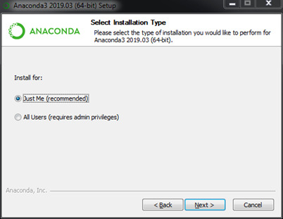
In select installation type, choose “Just Me (Recommended)” and choose the location where you wish to save Anaconda and click on Next.

Step 4 In Advanced Options, checkmark both the boxes and click on Install. Once it is installed, click “Finish”.

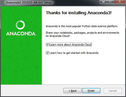
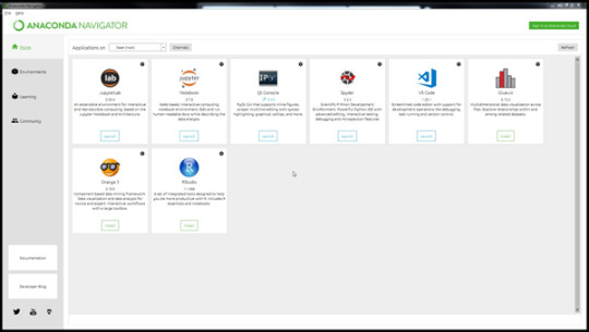
Now, you have successfully installed Anaconda on your system and it is ready to run. You can open the Anaconda Navigator and find other tools like Jupyter Notebook and Spyder IDE.

Once we have installed Anaconda, we will now move on to one of the most important components of the Python landscape, i.e. Python Libraries.

Note: Anaconda provides support for Linux as well as macOS. The installation details for the OS are provided on the official website in detail.

Libraries in Python

Libraries are a collection of reusable modules or functions which can be directly used in our code to perform a certain function without the necessity to write a code for the function. As mentioned earlier, Python has a huge collection of libraries which can be used for various functionalities like computing, machine learning, visualizations, etc. However, we will talk about the most relevant libraries required for coding trading strategies before actually getting started with Python. We will be required to:

import financial data,

perform numerical analysis,

build trading strategies,

plot graphs, and

perform backtesting on data.

For all these functions, here are a few most widely used libraries:

NumPy – NumPy or NumericalPy, is mostly used to perform numerical computing on arrays of data. The array is an element which contains a group of elements and we can perform different operations on it using the functions of NumPy.

Pandas – Pandas is mostly used with DataFrame, which is a tabular or a spreadsheet format where data is stored in rows and columns. Pandas can be used to import data from Excel and CSV files directly into the Python code and perform data analysis and manipulation of the tabular data.

Matplotlib – Matplotlib is used to plot 2D graphs like bar charts, scatter plots, histograms etc. It consists of various functions to modify the graph according to our requirements too.

TA-Lib – TA-Lib or Technical Analysis library is an open-source library and is extensively used to perform technical analysis on financial data using technical indicators such as RSI (Relative Strength Index), Bollinger bands, MACD etc. It not only works with Python but also with other programming languages such as C/C++, Java, Perl etc. Here are some of the functions available in TA-Lib:

BBANDS - For Bollinger Bands,

AROONOSC - For Aroon Oscillator,

MACD - For Moving Average Convergence/Divergence,

RSI - For Relative Strength Index.

Read about more such functions here.

Zipline – Zipline is a Python library for trading applications that power the Quantopian service mentioned above. It is an event-driven system that supports both backtesting and live trading.

These are but a few of the libraries which you will be using as you start using Python to perfect your trading strategy. To know about the myriad number of libraries in more detail, you can browse through this blog on Popular Python Trading platforms.

How to import data to Python?

This is one of the most important questions which needs to be answered before getting started with Python trading, as without data there is nothing you can go ahead with. Financial data is available on various online websites. This data is also called as time-series data as it is indexed by time (the timescale can be monthly, weekly, daily, 5 minutely, minutely, etc.). Apart from that, we can directly upload data from Excel sheets too which are in CSV format, which stores tabular values and can be imported to other files and codes. Now, we will learn how to import both time-series data and data from CSV files through the examples given below.

Importing Time Series Data

Here’s an example on how to import time series data from Yahoo finance along with the explanation of the command in the comments:

Note: In Python, we can add comments by adding a ‘#’ symbol at the start of the line.

To fetch data from Yahoo finance, you need to first pip install yfinance.

!pip install yfinance

You can fetch data from Yahoo finance using the download method.

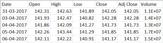
# Import yfinance import yfinance as yf # Get the data for stock Facebook from 2017-04-01 to 2019-04-30 data = yf.download('AAPL', start="2017-04-01", end="2019-04-30") # Print the first five rows of the data data.head()

Output:

Now, let’s look at another example where we can import data from an existing CSV file:

# Import pandas import pandas as pd # Read data from csv file data = pd.read_csv('FB.csv') data.head()

Creating a trading strategy and backtesting in Python

One of the simplest trading strategies involves Moving averages. But before we dive right into the coding part, we shall first discuss the mechanism on how to find different types of moving averages and then finally move on to one moving average trading strategy which is moving average convergence divergence, or in short, MACD. Let’s start with a basic understanding of moving averages.

What are Moving Averages?

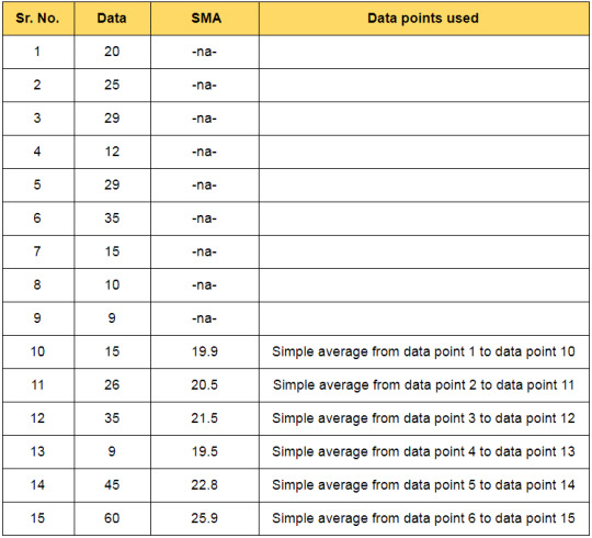
Moving Average also called Rolling average, is the mean or average of the specified data for a given set of consecutive periods. As new data becomes available, the mean of the data is computed by dropping the oldest value and adding the latest one. So, in essence, the mean or average is rolling along with the data, and hence the name ‘Moving Average’. An example of calculating the simple moving average is as follows: Let us assume a window of 10, ie n = 10

In the financial market, the price of securities tends to fluctuate rapidly and as a result, when we plot the graph of the price series, it is very difficult to predict the trend or movement in the price of securities. In such cases moving average will be helpful as it smoothens out the fluctuations, enabling traders to predict movement easily. Slow Moving Averages: The moving averages with longer durations are known as slow-moving averages as they are slower to respond to a change in trend. This will generate smoother curves and contain lesser fluctuations. Fast Moving Averages: The moving averages with shorter durations are known as fast-moving averages and are faster to respond to a change in trend.

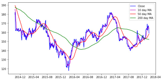
Consider the chart shown above, it contains:

the closing price of a stock IBM (blue line),

the 10-day moving average (magnum line),

the 50-day moving average (red line) and

the 200-day moving average (green line).

It can be observed that the 200-day moving average is the smoothest and the 10-day moving average has the maximum number of fluctuations. Going further, you can see that the 10-day moving average line is a bit similar to the closing price graph.

Types of Moving Averages

There are three most commonly used types of moving averages, the simple, weighted and the exponential moving average. The only noteworthy difference between the various moving averages is the weights assigned to data points in the moving average period. Let’s understand each one in further detail:

Simple Moving Average (SMA)

A simple moving average (SMA) is the average price of a security over a specific period of time. The simple moving average is the simplest type of moving average and calculated by adding the elements and dividing by the number of time periods. All elements in the SMA have the same weightage. If the moving average period is 10, then each element will have a 10% weightage in the SMA. The formula for the simple moving average is given below:

SMA = Sum of data points in the moving average period / Total number of periods

Exponential Moving Average (EMA)

The logic of exponential moving average is that latest prices have more bearing on the future price than past prices. Thus, more weight is given to the current prices than to the historic prices. With the highest weight to the latest price, the weights reduce exponentially over the past prices. This makes the exponential moving average quicker to respond to short-term price fluctuations than a simple moving average. The formula for the exponential moving average is given below:

EMA = (Closing price - EMA*(previous day)) x multiplier + EMA*(previous day)

Weightage multiplier = 2 / (moving average period +1)

Weighted Moving Average (WMA)

The weighted moving average is the moving average resulting from the multiplication of each component with a predefined weight. The exponential moving average is a type of weighted moving average where the elements in the moving average period are assigned an exponentially increasing weightage. A linearly weighted moving average (LWMA), generally referred to as weighted moving average (WMA), is computed by assigning a linearly increasing weightage to the elements in the moving average period. Now that we have an understanding of moving average and their different types, let’s try to create a trading strategy using moving average.

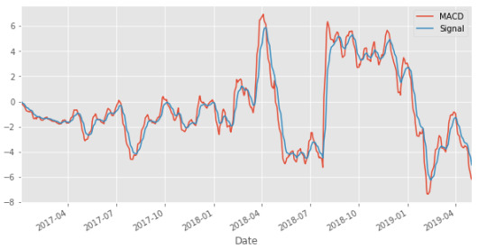
Moving Average Convergence Divergence (MACD)

Moving Average Convergence Divergence or MACD was developed by Gerald Appel in the late seventies. It is one of the simplest and effective trend-following momentum indicators. In MACD strategy, we use two series, MACD series which is the difference between the 26-day EMA and 12-day EMA and signal series which is the 9 day EMA of MACD series. We can trigger the trading signal using MACD series and signal series.

When the MACD line crosses above the signal line, then it is recommended to buy the underlying security.

When the MACD line crosses below the signal line, then a signal to sell is triggered.

Implementing the MACD strategy in Python

Import the necessary libraries and read the data

# Import pandas import pandas as pd # Import matplotlib import matplotlib.pyplot as plt plt.style.use('ggplot') # Read the data data = pd.read_csv('FB.csv', index_col=0) data.index = pd.to_datetime(data.index, dayfirst=True) # Visualise the data plt.figure(figsize=(10,5)) data['Close'].plot(figsize=(10,5)) plt.legend() plt.show()

Calculate and plot the MACD series which is the difference 26-day EMA and 12-day EMA and signal series which is 9 day EMA of the MACD series.

# Calculate exponential moving average data['12d_EMA'] = data.Close.ewm(span=12).mean() data['26d_EMA'] = data.Close.ewm(span=26).mean() data[['Close','12d_EMA','26d_EMA']].plot(figsize=(10,5)) plt.show()

# Calculate MACD data['MACD'] = data['26d_EMA'] - data['12d_EMA'] # Calculate Signal data['Signal'] = data.MACD.ewm(span=9).mean() data[['MACD','Signal']].plot(figsize=(10,5)) plt.show()

Create a trading signal When the value of MACD series is greater than signal series then buy, else sell.

# Import numpy import numpy as np # Define Signal data['trading_signal'] = np.where(data['MACD'] > data['Signal'], 1, -1)

Create and calculate the strategy return

# Calculate Returns data['returns'] = data.Close.pct_change() # Calculate Strategy Returns data['strategy_returns'] = data.returns * data.trading_signal.shift(1) # Calculate Cumulative Returns cumulative_returns = (data.strategy_returns + 1).cumprod()-1 # Plot Strategy Returns cumulative_returns.plot(figsize=(10,5)) plt.legend() plt.show()

Evaluation of a trading strategy

So far, we have created a trading strategy as well as backtested it on historical data. But does this mean it is ready to be deployed in the live markets? Well, before we make our strategy live, we should understand its effectiveness, or in simpler words, the potential profitability of the strategy. While there are many ways to evaluate a trading strategy, we will focus on the following,

Annualised return,

Annualised volatility, and

Sharpe ratio.

Let’s understand them in detail as well as try to evaluate our own strategy based on these factors:

1. Annualised Return or Compound Annual Growth Rate (CAGR)

To put it simply, CAGR is the rate of return of your investment which includes the compounding of your investment. Thus it can be used to compare two strategies and decide which one suits your needs. Calculating CAGR CAGR can be easily calculated with the following formula:

CAGR = [(Final value of investment /Initial value of investment)^(1/number of years)] - 1

For example, we invest in 2000 which grows to 4000 in the first year but drops to 3000 in the second year. Now, if we calculate the CAGR of the investment, it would be as follows:

CAGR = (3000/2000)^(½) - 1 = 0.22 = 22%

For our strategy, we will try to calculate the daily returns first and then calculate the CAGR. The code, as well as the output, is given below: In[]

# Total number of trading days in a year is 252 trading_days = 252 # Calculate CAGR by multiplying the average daily returns with number of trading days annual_returns = ((1 + data.returns.mean())**(trading_days) - 1)*100 'The CAGR is %.2f%%' % annual_returns

Out []:

'The CAGR is 30.01%'

2. Annualised Volatility

Before we define annualised volatility, let’s understand the meaning of volatility. A stock’s volatility is the variation in the stock price over a period of time. For the strategy, we are using the following formula:

Annualised Volatility = square root (trading days) * square root (variance)

The code, as well as the output, is given below: In[]

# Calculate the annualised volatility annual_volatility = data.returns.std() * np.sqrt(trading_days) * 100 'The annualised volatility is %.2f%%' % annual_volatility

Out []:

'The annualised volatility is 30.01%'

3. Sharpe Ratio

Sharpe Ratio is basically used by investors to understand the risk taken in comparison to the risk-free investments, such as treasury bonds etc. The sharpe ratio can be calculated in the following manner:

Sharpe ratio = [r(x) - r(f)] / δ(x)

Where,

r(x) = annualised return of investment x r(f) = Annualised risk free rate δ(x) = Standard deviation of r(x)

The Sharpe Ratio should be high in case of similar or peers. The code, as well as the output, is given below: In[]

# Assume the annual risk-free rate is 6% risk_free_rate = 0.06 daily_risk_free_return = risk_free_rate/trading_days # Calculate the excess returns by subtracting the daily returns by daily risk-free return excess_daily_returns = data.returns - daily_risk_free_return # Calculate the sharpe ratio using the given formula sharpe_ratio = (excess_daily_returns.mean() / excess_daily_returns.std()) * np.sqrt(trading_days) 'The Sharpe ratio is %.2f' % sharpe_ratio

Out[]:

'The Sharpe ratio is 0.68'

Python Books and References

Python Basics: With Illustrations From The Financial Markets

A Byte of Python

A Beginner’s Python Tutorial

Python Programming for the Absolute Beginner, 3rd Edition

Python for Data Analysis, By Wes McKinney

Conclusion

Python is widely used in the field of machine learning and now trading. In this article, we have covered all that would be required for getting started with Python. It is important to learn it so that you can code your own trading strategies and test them. Its extensive libraries and modules smoothen the process of creating machine learning algorithms without the need to write huge codes. To start learning Python and code different types of trading strategies, you can select the “Algorithmic Trading For Everyone” learning track on Quantra. Disclaimer: All data and information provided in this article are for informational purposes only. QuantInsti® makes no representations as to accuracy, completeness, currentness, suitability, or validity of any information in this article and will not be liable for any errors, omissions, or delays in this information or any losses, injuries, or damages arising from its display or use. All information is provided on an as-is basis.

Trading via QuantInsti http://bit.ly/2Zi7kP2 August 26, 2019 at 04:14AM

#IFTTT #Feedly

0 notes

lindarifenews · 6 years ago

Text

Brands can better understand users on third-party sites by using a keyword overlap analysis

If you are a manufacturer selling on your own site as well as on retail partners, it is likely you don’t have visibility into who is buying your products or why they buy beyond your own site. More importantly, you probably don’t have enough insights to improve your marketing messaging.

One technique you can use to identify and understand your users buying on third-party websites is to track your brand through organic search. You can then compare the brand searches on your site and the retail partner, see how big the overlap is, how much of the overlapping keywords you rank above the retailer and vice versa. More importantly, you can see if you are appealing to different audiences or competing for the same ones. Armed with these new insights, you could restructure your marketing messaging to unlock new audiences you didn’t tap into before.

In previous articles, I’ve covered several useful data blending examples, but in this one, we will do something different. We will do a deeper dive into just one data blending example and perform what I call a cross-site branded keyword overlap analysis. As you will learn below, this type of analysis will help us understand your users buying on third-party retailer partners.

In the Venn diagram above, you can see an example of visualization we will put together in this article. It represents the number of overlapping keywords in organic search for the brand “Tommy Hilfiger” between their main brand site and Macy’s, a retail partner.

We recently had to perform this analysis for one of our clients and our findings surprised us. We discovered that with 60% of our client’s organic SEO traffic coming from branded searches, as much as 30% of those searches were captured by four retailer partners that also sell their products.

Armed with this evidence and with the knowledge that selling through their retail partners still made business sense, we provided guidance on how to improve their brand searches so they can compete more effectively, and change their messaging to appeal to a different customer than the one that buys from the retailers.

After my team conducted this analysis manually and I saw how valuable it is, I set out to automate the whole process in Python so we could easily reproduce it for all our manufacturing clients. Let me share the code snippets I wrote here and walk you over their use.

Pulling branded organic search keywords

I am using the Semrush API to collect the branded keywords from their service. I created a function to take their response and return a pandas data frame. This function simplifies the process of collecting data for multiple domains.

Here is the code to get organic searches for “Tommy Hilfiger” going to Macy’s.

Here is the code to get organic searches for “Tommy Hilfiger” going to Tommy Hilfiger directly.

Visualizing the branded keyword overlap

After we pull the searches for “Tommy Hilfiger” from both sites, we want to understand the size of the overlap. We accomplish this in the following lines of code:

We can quickly see that the overlap is significant, with 4601 keywords in common, 515 unique to Tommy Hilfiger, and 125 unique to Macy’s.

Here is the code to visualize this overlap as the Venn diagram illustrated above.

Who ranks better for the overlapping keywords?

The most logical next question you would want to ask is that given how significant the overlap is, who commands more higher rankings for those. How can we figure this out? With data blending of course!

First, as we learned in my first data blending article, we will merge the two data frames, and we will use an inner join to keep only the keywords common in the two sets.

When we merge data frames and they have the same columns, they are repeated and the first columns include _x at the end and the second one includes _y. So, Macy’s columns end with _x.

Here is how we create a new data frame with the overlapping branded keywords where Macy’s ranks higher.

Here is the corresponding data frame where Tommy Hilfiger ranks higher.

Here we can see that while the overlap is big, Tommy ranks higher for many more branded keywords than Macy’s (3,173 vs. 1,075). So, is Tommy doing better? Not quite!

As you remember, we also pulled traffic numbers from the API. In the next snippet of code, we will check which keywords are pulling more traffic.

Surprisingly, we see that, while Macy’s performs better for fewer keywords than Tommy Hilfiger, when we add up the traffic, Macy’s attracts more visitors (75,026 vs. 66,415).

As you can see, sweating the details matters a lot in this type of analysis!

How different are the audiences

Finally, let’s use the branded keywords unique to each site to learn any differences in the audiences that visit each site. We will simply strip the branded phrase from the keywords and create word clouds to understand them better. When we remove the branded phrase “Tommy Hilfiger,” we are left with the additional qualifiers that users use to indicate their intention.

I created a function to create and display the word clouds. Here is the code:

Here is the word cloud with the most popular words left after you remove the phrase “Tommy Hilfiger” from Macy’s keywords.

Here is the corresponding word cloud when you do the same for the Tommy Hilfiger ones.

The main difference I see is people looking for Tommy Hilfiger products in Macy’s have specific products in mind, like boots and curtains, while when it comes to the brand site, people primarily have the outlets in mind. This might be an indicator that they intend to visit the store vs. trying to purchase online. This may also indicate that people going to brand site are bargain hunters while the ones going to Macy’s might not be. These are very interesting and powerful insights!

Given these insights, Tommy Hilfiger could review the SERPS and compare the difference in the messaging between Macy’s and their brand site and adjust it to appeal to their unique audience’s interests.

The post Brands can better understand users on third-party sites by using a keyword overlap analysis appeared first on Search Engine Land.

Brands can better understand users on third-party sites by using a keyword overlap analysis published first on https://likesfollowersclub.tumblr.com/

0 notes

andreacaskey · 6 years ago